Introduction

A friend of mine approached me to analyze a vehicle in his company, he wanted to use a data-driven approach to determine the cost of ownership of the vehicle in the fleet. Buying the vehicle was easy. It was affordable and had very low mileage at the time of purchase and had 4 more years left on the certificate of entitlement. What about the operating costs of the vehicle? Drivers record the usage data such as distance travelled and fuel consumption in a logbook. 

A single vehicle should be easy to visualise. But what about a fleet of vehicles? This is a particular issue for logistics and delivery services that drive e-commerce. A logistics company needs to manage a fleet of vehicles of different models, load capacities and ages.

I decided to run some numbers in Python for a simple econometric experiment using that vehicle dataset provided, but the methods I describe in this article are applicable to anyone interested in vehicle or asset cost management. Simply put, econometrics is the application of statistical models to test economic theories and is a branch of data science. Instead of experimental data, observed data are used to determine the effects of random events.

In machine learning, time series analysis is slightly different from normal regression or classification problems. Time series regression helps us understand the relationship between variables over time and predict future values. I wrote several time series prediction scripts in Python and explored several multivariate algorithms for modelling time series, examining the following algorithms: Autoregressive Integrated Moving Average (ARIMAx), Generalized AutoRegressive Conditional Heteroskedasticity (GARCH), Least absolute shrinkage and selection operator (LASSO), PROPHET, RIDGE, Support Vector Regression (SVR) and k-nearest neighbors (kNN). 

There was no particular reason for choosing the machine learning algorithms, but these are just the common ones and there are numerous other models that can be explored which I will discuss later. 

The algorithms used in this study are not the most advanced, but this is the first time I have dealt with time series, and the goal of this paper is to explore a data-driven approach that can help one make enterprise-level decisions about which vehicle to use on which route and what type of maintenance to perform (e.g., tyre changes, oil changes) and how this affects the life of the vehicle and whether I should maintain a well-functioning vehicle or buy a new vehicle.

The dataset

Date	Item	Distance (+km)	Fuel (L)	Cost
8/1/2021	Purchase of vehicle			$ 25,000.00
8/1/2021	Accessories			$ 19.55
8/1/2021	Insurance			$ 872.75
8/1/2021	Accessories			$ 27.25
8/2/2021	Parking			$ 1,422.70
8/7/2021	Accessories			$ 12.47
8/9/2021	Petrol	365	33.62	$ 54.00
8/14/2021	Parking			$ 50.00
8/14/2021	Maintenance			$ 620.00
8/15/2021	Petrol	161		$ 94.00
22/8/2021	Parking			$ 20.00
22/8/2021	Petrol	264	41.5	$ 74.00
28/8/2021	Parking			$ 52.00
28/8/2021	Petrol	287	21.3	$ 72.00
28/8/2021	Parking			$ 10.00
4/9/2021	Petrol	266	31.5	$ 72.00
9/11/2021	Petrol	249	24.59	$ 68.50
9/13/2021	Parking			$ 100.00
9/16/2021	Maintenance			$ 265.27
9/16/2021	Road Tax			$ 378.00
9/17/2021	Petrol	288	47.22	$ 73.00
9/25/2021	Parking			$ 30.00

The above table shows a typical record of operations for two months. The record of expenditures for the vehicle was straightforward, a simple distance and expense log. There were typical expenses for fuel or a sudden large bill for renewal of a seasonal parking space or road tax, but all in all the record is fairly linear and also a typical log for any driver in the courier business. I had to wait a while before I could start any kind of analysis. Now I have about 100 data points from August 2021 to December 2022, a little over a year.

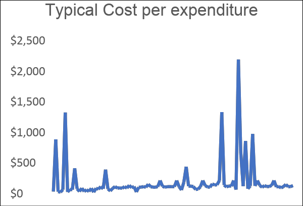
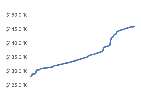
Figure 1 So this is how the data looks like over a year, the first graph on the left shows the amount of each expense and on the right is a cumulative expense which represents the lifetime cost of the vehicle.

The figure above shows two diagrams. The diagram on the left shows the amount of each expense, such as a typical tank of gas or a parking fee, and the largest expense was replacing all tyres and rims with new tyres. The chart on the right shows the cumulative cost over time.

Figure 2 Data importing into an array using the Python Numpy Library

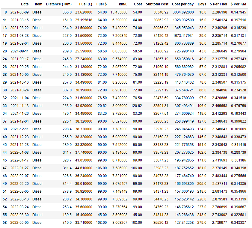
Figure 3 Dataframe recording the fuel consumption and distance travelled. 

I’m interested in determining the total cost of ownership of my vehicle to see if I can make some data-driven decisions to increase the value of the vehicle. This could include making certain changes to improve fuel economy. In my case, I recorded how far I drove, how often I filled up with gas, and what my car expenses were. What I’m interested in is the cost per day at the end of the vehicle’s life, both in terms of fuel consumption and total cost of ownership.

The algorithms

Let’s introduce some algorithms explored.

1. ARIMA. This nifty algorithm is an acronym for AutoRegression (AR) – where the dependent relationship between an observation and a specified number of previous observations, Integrated (I), the use of differencing raw observations (e.g., subtracting an observation from an observation in the previous time step) to make the time series stationary, and Moving Average (MA) – where the dependence between an observation and a residual error from a moving average model applied to lagged observations. Variants of this algorithm include a seasonality component denoted by “s” – SARIMA or SARIMAX. A very good textbook description can be found here and sample code here and here.  
2. GARCH. AutoRegressive Conditional Heteroskedasticity is commonly used in modelling stock-trading data that exhibit time-varying volatility clusters, the algorithm describes the variance of the current data point as a function of the actual magnitudes of the error terms of the previous periods. GARCH is a generalized version of ARCH, a helpful Youtube video can be found here.
3. LASSO (least absolute shrinkage and selection operator) is a method of regression analysis that performs both variable selection and regularization. Here’s a video describing this algorithm.
4. RIDGE. Is a regression algorithm similar to linear regression but with bias introduced, this gives us a reduction in variance, and by reducing fit we can have better long term predictions, more here. 
5. PROPHET. Now this is a new algorithm to me, it is an additive regression model with a piecewise linear or logistic growth curve trend that accounts for seasonality, the algorithm was introduced by Sean J. Taylor and Ben Letham from Facebook in 2017, nicely explained here, here and here.
6. SVR. Support Vector Regression (SVR) is a regression technique that uses support vector machines (SVMs) to predict continuous values. Unlike KNN, SVR is a more advanced and sophisticated algorithm that uses a hyperplane to separate data points of one class from another. 
7. kNN. K Nearest Neighbours is a supervised ML algorithm used for classification and regression and does not assume any prior knowledge about the data. Simply put, all input data points are classified by a distance function to the next nearest data point. 

In addition to the links above, I found some useful repositories describing time-series analysis with the above algorithms here, here, here and here that was immensely valuable. 

Analysis and Discussion

There were about two years of data since the vehicle was purchased in August 2021. Data points were split into 80% – 20% for training and testing. The search for hyperparameters was done using the above models, and all models were then re-trained with the best hyperparameters and used for the test set extrapolating future predictions of weekly costs.

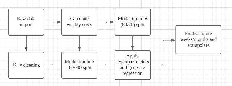
Figure 4 How the data was processed.

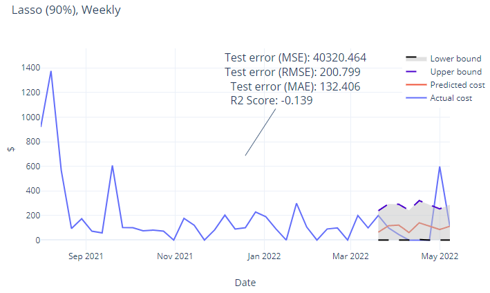
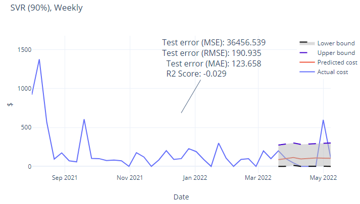
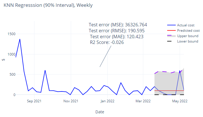
Figure 5 So with the typical costs over the year punched in to the various models, we can now predict what the costs will be like in the future when extrapolated. All the models showed a relatively linear extrapolation meaning that we don’t expect big expenses to move the needle much. 

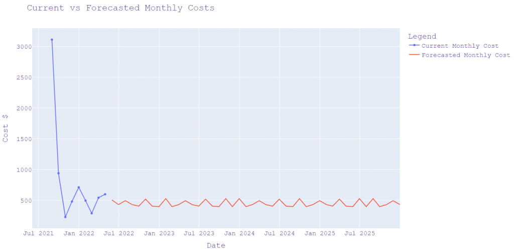
Figure 6 Current vs forecasted monthly costs – this is one model showing a linear expense of $450 per month, which tallied with real-world data. 

The various models predicted about $~500/month. The monthly predictions were close to real expenditures, I randomly checked a block of a few months. Apart from July 2022, which had a large payment for season parking, the other months were within expected limits. Each year an owner would have to expect a major expense for maintenance, road tax, etc., but these are not frequent expenses.

Month	March 2022	April 2022	May 2022	June 2022	July 2022	August 2022
actual Expense	$542	$597	$429	$600	$2,046	$564

Alright, we are getting somewhere. My first few attempts immediately showed the limitations or unsuitability of some of the models and the data that we have on hand. Some models such ARIMA and kNN showed a straight line and or reduction in projection. 

From the available data, current (to date) expenditures already exceed $50,000. Therefore, any prediction showing a lesser amount must be rejected. Since we already have two years of data – $11,924 in 2022 – and a reasonable monthly forecast of $500, a monthly average of $1,000 to cover the additional costs is not expected. 

This means that our model should realistically provide a lifetime vehicle cost forecast in the range of $10,000 to $15,000 per year and a lifetime total vehicle cost forecast of no more than $100,000. Any model that predicts less than $40,000 is wrong, and more than $100,000 is unrealistic.

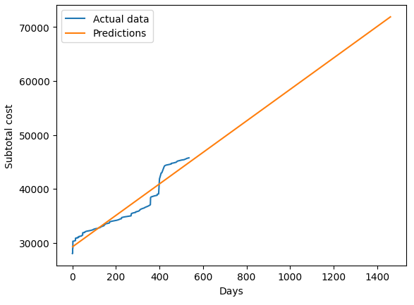
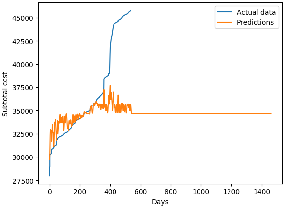
Figure 7 Left: The most rudimentary of extrapolations – a linear regression line shows a lifetime expenditure of the vehicle at $70,000, this is a reasonable estimate. Right: ARIMA predictions show a flat estimate, which is logically incorrect.

Now that we have some upper and lower limits, SARIMAX predicts a total lifetime cost of $51,360 and which is incorrect since it is less than the current total expenditure of the dataset with cost per day, whilst k-NN shows a flat line. These two models are rejected. Due to inconsistency in duration between data points. GARCH/ARCH refused to work properly – showing the limitations of these algorithms. As a classifier, kNN is unsuitable for such a time series application.

Results

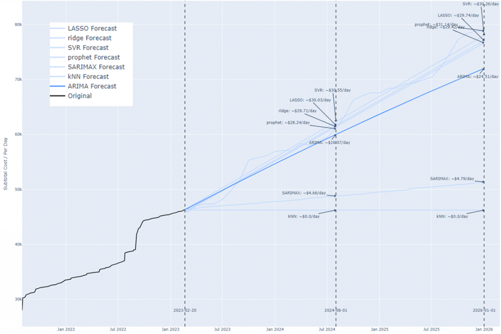
Figure 8 Forecasting total lifetime cost of the vehicle.

Model	Lifetime cost	Cost per day	Notes
PROPHET	$ 78,838	$ 31.14
SVR	$ 77,985	$ 30.26
LASSO	$ 77,073	$ 29.74
RIDGE	$ 76,642	$ 29.42
ARIMA	$ 72,008	$ 24.51
SARIMAX	$ 51,360	$ 4.79	Rejected
KNN	$ 46,226	$ 0.00	Rejected
GARCH	error	error	Rejected

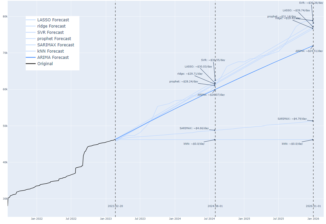
Figure 9 Forecasting total daily expenditure for ownership of the vehicle.

ARIMA, SVR, LASSO, RIDGE and PROPHET prediction limits of $72,000 to $78,000. Since the margin of error is very small, I could use various statistical techniques to calculate the confidence interval of the analysis, but at this point I’m satisfied with the predictions. The cost of the vehicle is about $30 per day – parking, taxes, maintenance, and fuel. This is reasonable.

In statistics, there are some other metrics that are used to determine the reliability of the model, but time series are a little different, traditional metrics like confidence interval, interquartile range, confusion matrices won’t really work because we don’t know if the future will actually be like this.

This paper proposes a method to estimate a reliability measure of the predictor a statistical method the authors call Statistical Semi-metric Space (SSMS). For simplicity, the PROPHET library generates an upper and lower boundary. 

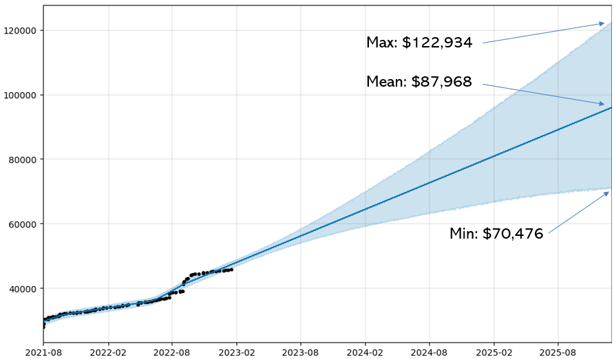
Figure 10 Upper and lower boundary estimates using PROPHET extrapolated from the existing dataset.

With that projection, we get an upper and lower boundary of the projection of $70,476 – $122,934 without any tweaking of the model – giving us a fairly large uncertainty boundary but still also reasonable in our projections, like an error-margin of estimation. I could manually adjust the hyperparameters of the PROPHET model such as the seasonality, growth points and uncertainty samples to make the projection upper and lower boundaries tighter but at this point all the projections point towards the same trajectory of a ~$80,000 expense over the remaining lifetime of the vehicle, which gives us an acceptable range of $30±1.24 cost per day. Budgeting a little buffer over the projection of future expenses wouldn’t hurt. 

Conclusion, comments and future work

This mini project took a surprisingly longer than expected. But I must say very satisfying. In the future I could apply an intangible valuation aspect of owning a vehicle such as convenience over public-transport or private-hire vehicles. In the future I would like to look into more recent and advanced time-series algorithms such as Deep-XF, ETSformer, N-Beats (Neural Basis Expansion),  N-Hits (Neural Hierarchical Interpolation for Time Series Forecasting), Temporal Fusion Transformers (TFT), Informers and Autoformers.

Epilogue

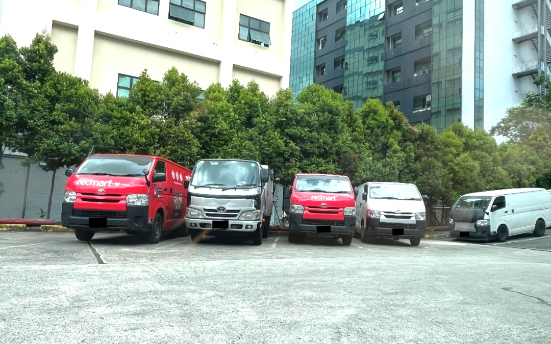
My buddy bought more of the same vans and a drink for me. 

Disclaimer 

All the work represented in this article are of my own investigation and the numbers should be taken as an exercise and not any form of formal financial or fiduciary advisory. Contact me if you would like to discuss econometric assessments or investigation services into your business problem.